Make a Technical-Illustration Hurricane Data Poster
Build a vintage scientific plate in Lopsy, with a duotone satellite view, a hatched hurricane cross-section, a bar chart and a line chart, all with masks, groups and live type.
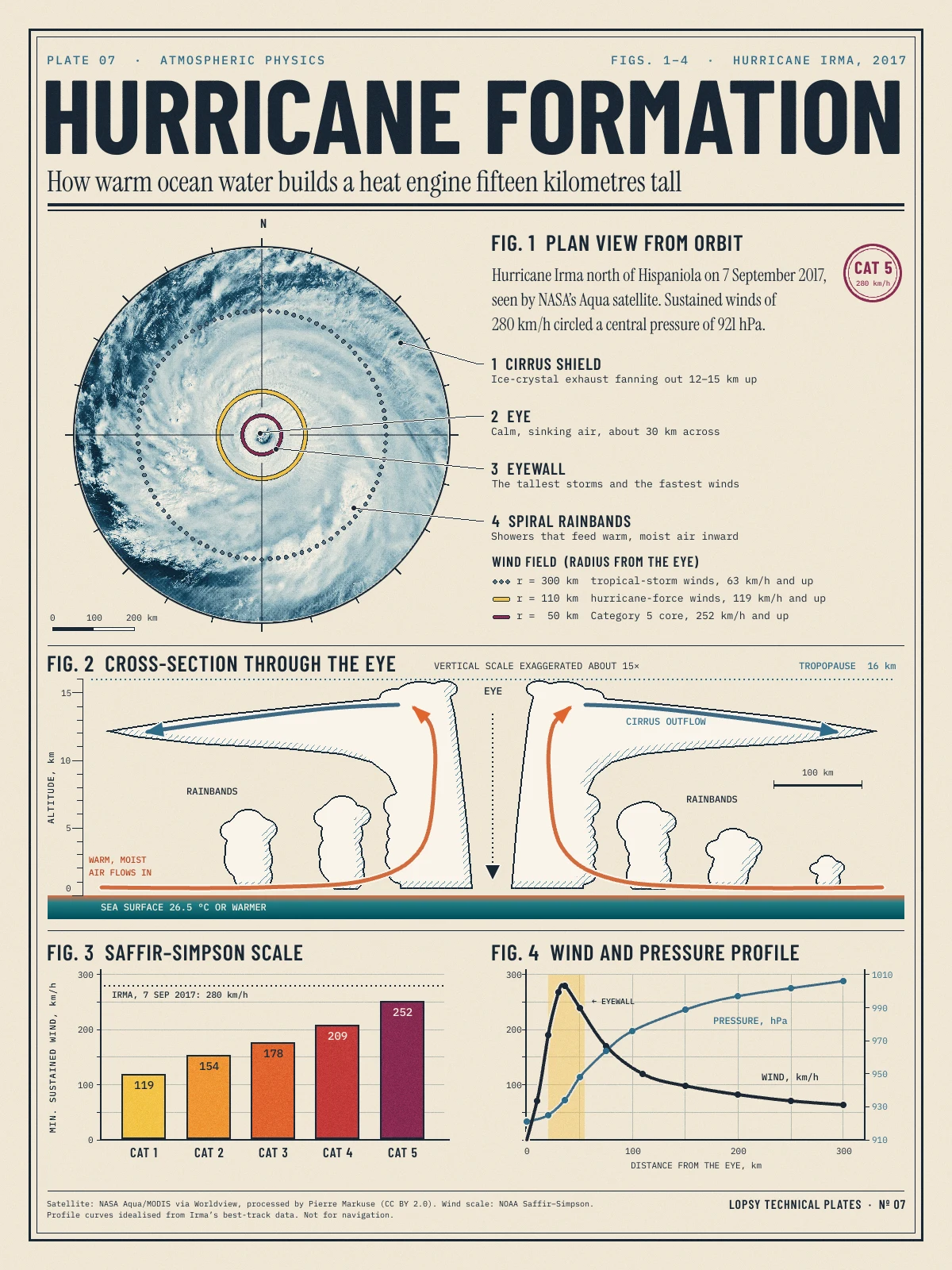
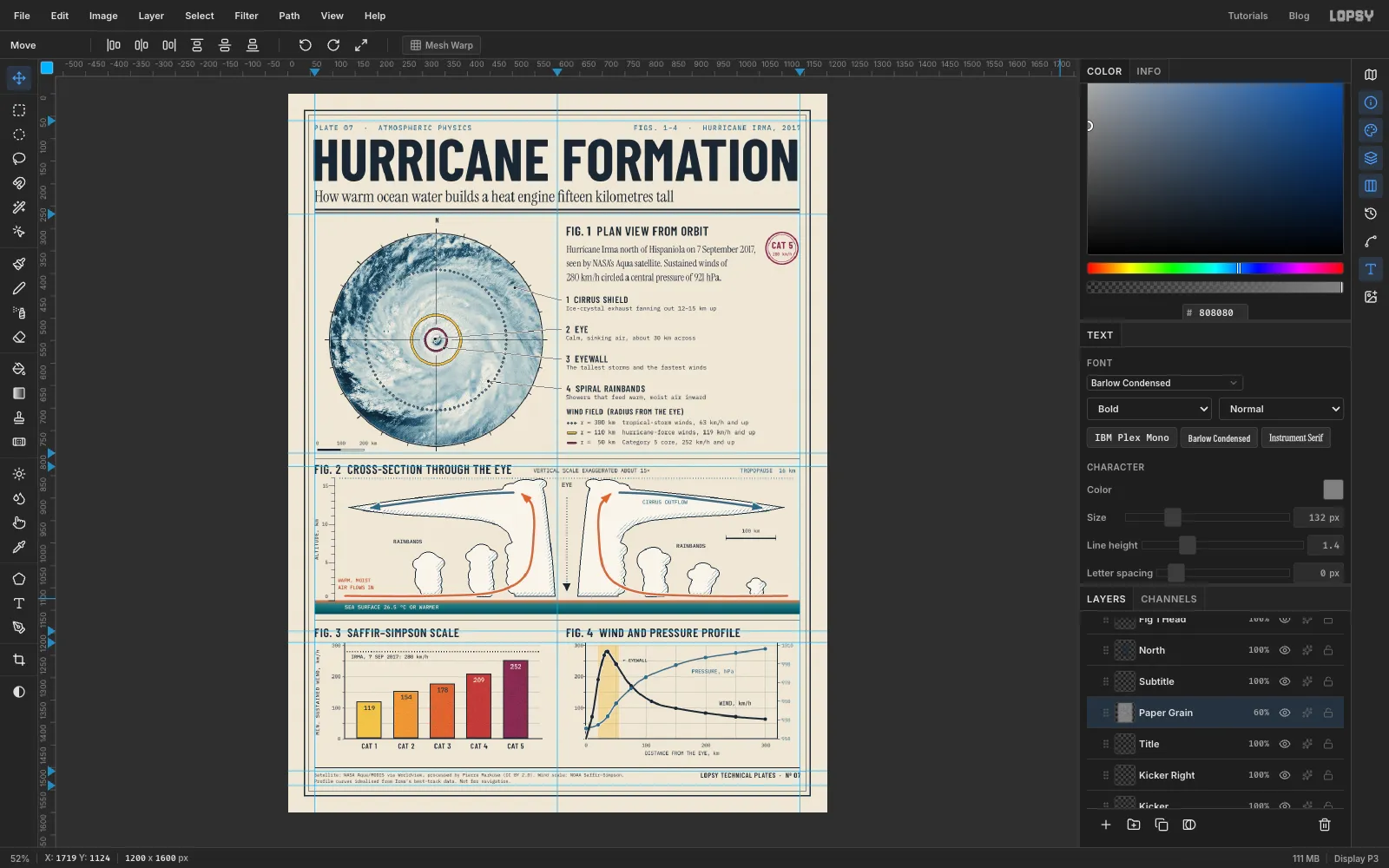
Old science textbooks explained the world in plates: one sheet, a few numbered figures, fine ink lines, and a caption under each. This tutorial builds one of those plates about how a hurricane works. It has four figures that tell one story:
- Fig. 1 is a real satellite photo of Hurricane Irma, turned into a two-colour print with rings showing how far its winds reach.
- Fig. 2 cuts the storm in half so you can see the warm air going in at the bottom, up the eyewall and out at the top.
- Fig. 3 is a bar chart of the Saffir–Simpson scale.
- Fig. 4 plots wind and pressure against distance from the eye.
You'll need the satellite photo. It's Hurricane Irma Sep 7 Aqua MODIS Eye Zoom.jpg) by Pierre Markuse, from NASA data, under CC BY 2.0. It has a zoomed inset in the top right corner and a caption strip along the bottom. Before you start, crop it to a square about 1,100 px across with the eye in the middle, so the inset and the caption stay out. You can open the photo in Lopsy, crop it with the Crop tool (C) and export it, or use any image viewer. The poster credits the photo in its footer, and yours should too.
Along the way you'll use:
- guides, the grid with Snap, and exact-corner marquees
- a dropped photo, a Cmd-drag scale and a layer mask
- Group Layers plus a Gradient Map adjustment for the duotone
- Duplicate Layer, Halftone, Multiply and Overlay
- the Brush with Radial Symmetry for compass ticks and a dotted ring
- Fill → Shrink → Delete for crisp rings and frames
- the Lasso and Elliptical Marquee with Shift (add) and Alt (subtract)
- Define Pattern and Fill with Pattern for hatching
- the Pen tool, stroked with Enter, for smooth arrows and curves
- Stroke layer effects for outlines and paper halos
- live text in Barlow Condensed, IBM Plex Mono and Instrument Serif, including two labels turned 90°
- Group Layers and an arrow-key nudge on the grid
The palette is navy ink on warm paper, with the storm categories as the only strong colour:
-
Paper
-
ink
-
card
-
Rule blue
-
dot grey
-
hairlines
-
Duotone
-
Categories
-
Sea
-
Cloud
-
inflow label
-
Set up the paper and guides
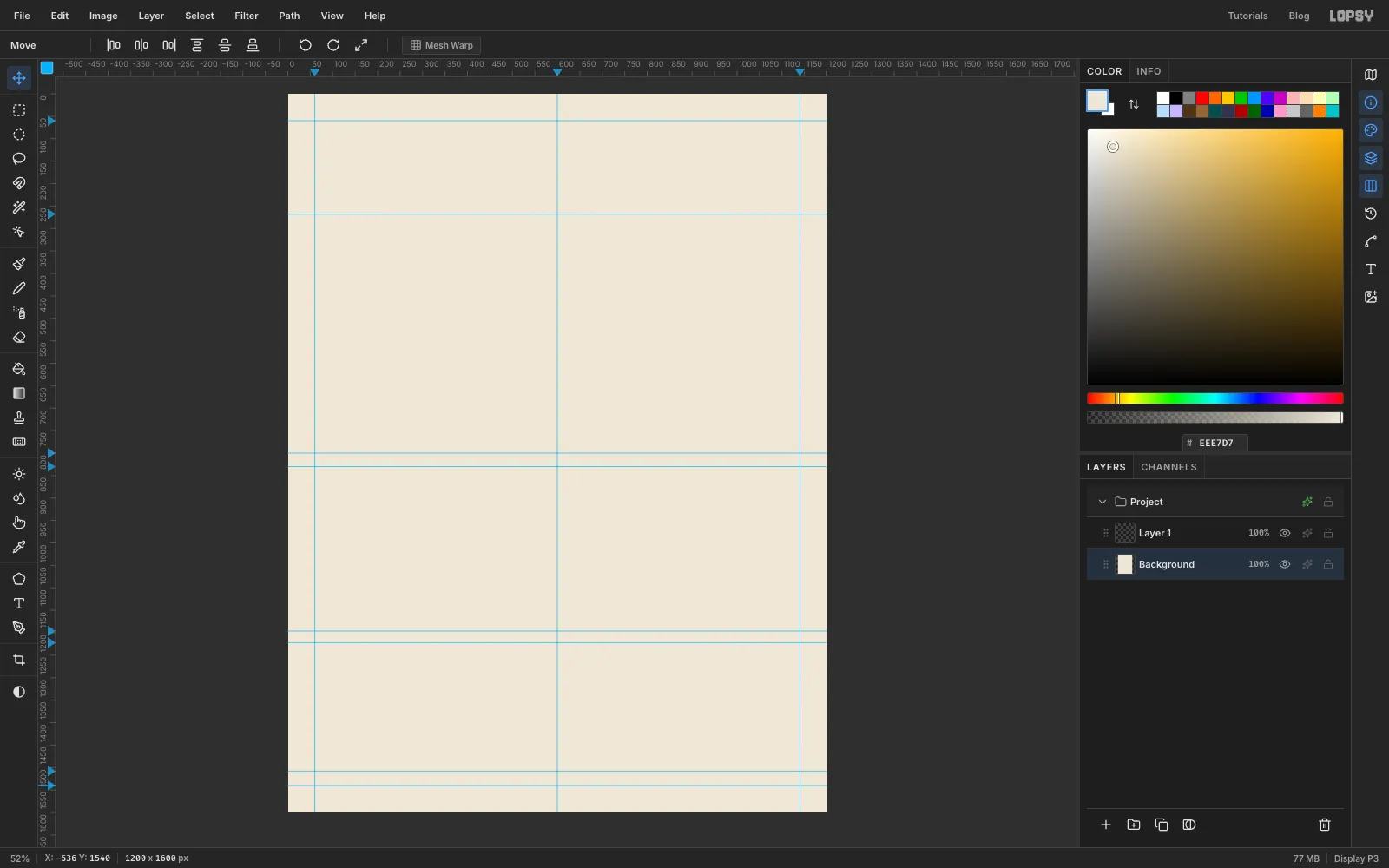
Open Lopsy and create a new document 1200 wide by 1600 tall.
- Select Background, set the foreground colour to and choose Edit → Fill. With nothing selected it fills the whole layer.
- Click the top ruler at
60,600and1140for the two side margins and the centre line. - Click the left ruler at
60and268for the top margin and the bottom of the header. I also dropped a few more horizontal guides lower down as rough markers for the figure bands. Their exact heights don't matter.
-
Add grain and a double frame
Real paper is never perfectly flat. With Background still selected, choose Filter → Add Noise…, set Amount to
4, pick Mono and Gaussian, and click Apply.Rename Layer 1 to
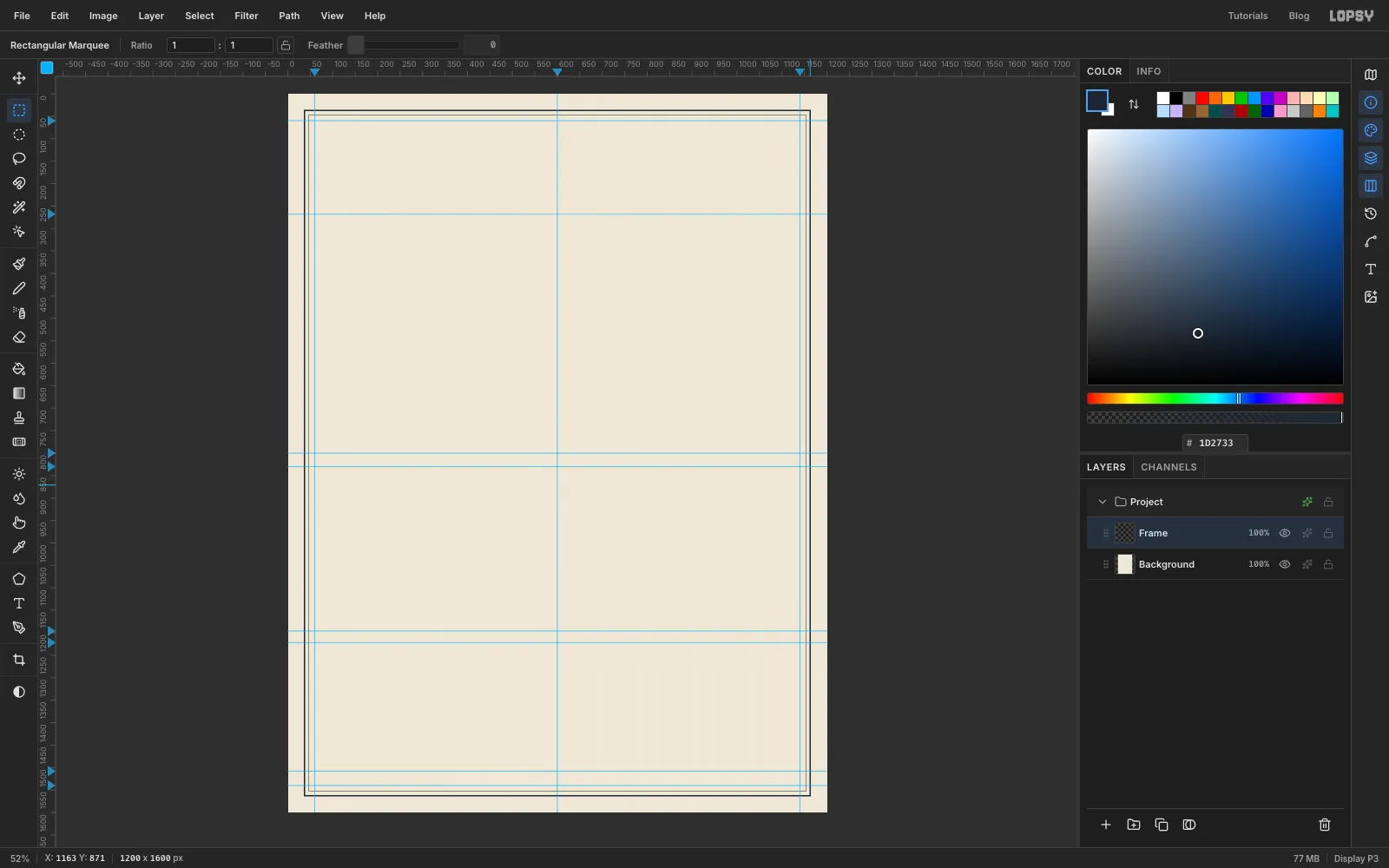
Frameby double-clicking its name. The frame is two rings, each made with the same trick: fill a rectangle, shrink the selection, then delete the middle.- Make an exact-corner selection from
36, 36to1164, 1564. Set the foreground to and choose Edit → Fill. - Choose Select → Shrink…, set Amount to
3, click Apply, and press Delete. You're left with a 3 px ink border. - Repeat with a selection from
46, 46to1154, 1554and a shrink of1for the thin inner rule. - Deselect with Cmd+D.
- Make an exact-corner selection from
-
Drop in the satellite photo and scale it down
Click Background so the photo will land just above it, then drag your cropped photo file onto the canvas. It arrives as a new layer in the top left corner, already selected. Rename it
Satellite.The plan view will be a circle 470 px across. To fit a good part of the storm inside that circle, scale the photo down to 561 px wide: hold Cmd and drag its bottom-right handle up and to the left. Cmd keeps it square. Watch the status bar and let go at about
561, 561. Press Enter to apply, then Cmd+D.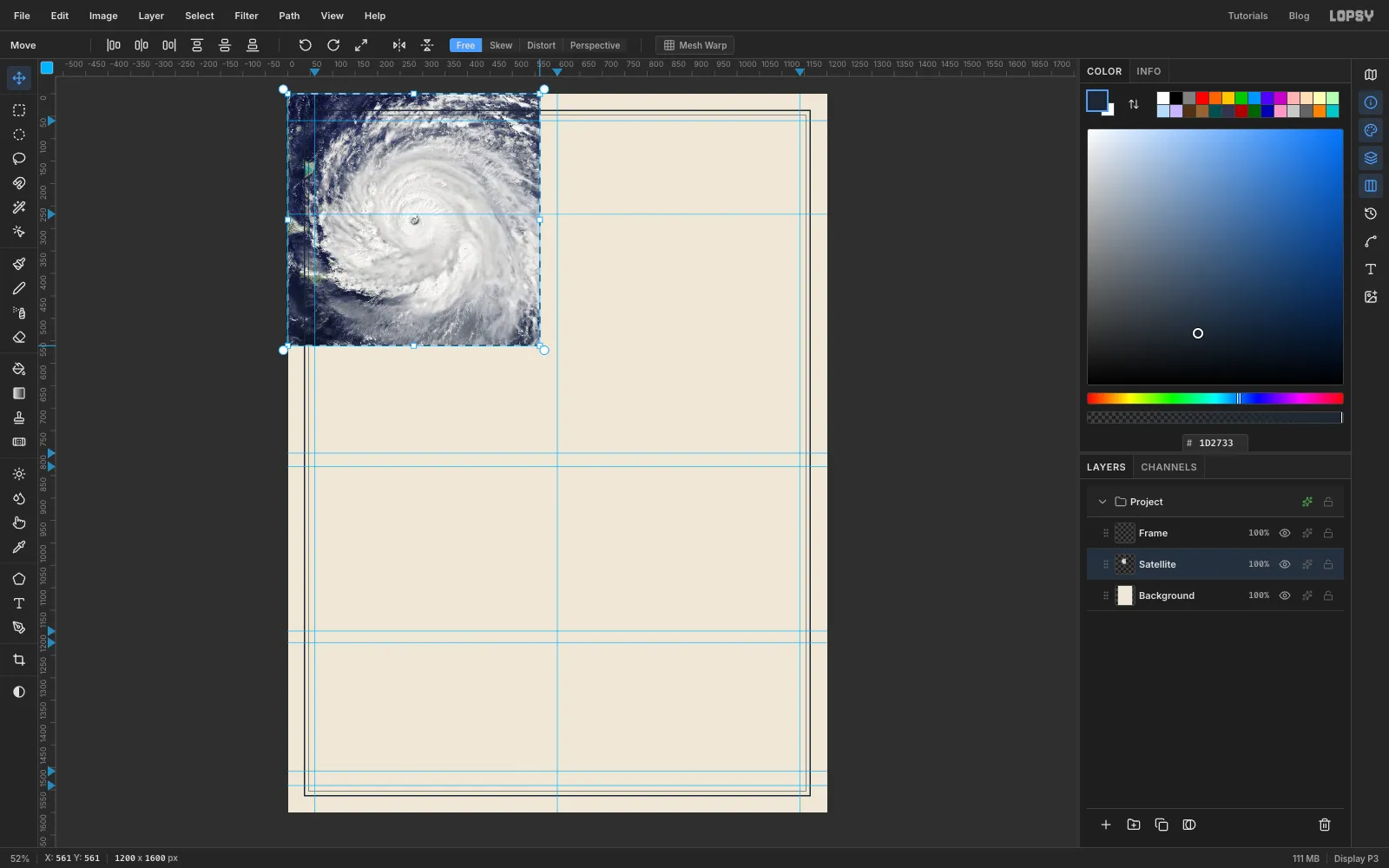
-
Centre the photo on the plan view
Pick the Move tool (V) and drag the photo until its centre, the eye, sits at about
330, 548. That puts the plan view's centre 330 px from the left edge, which leaves room for callouts on the right. Deselect if a selection is left behind.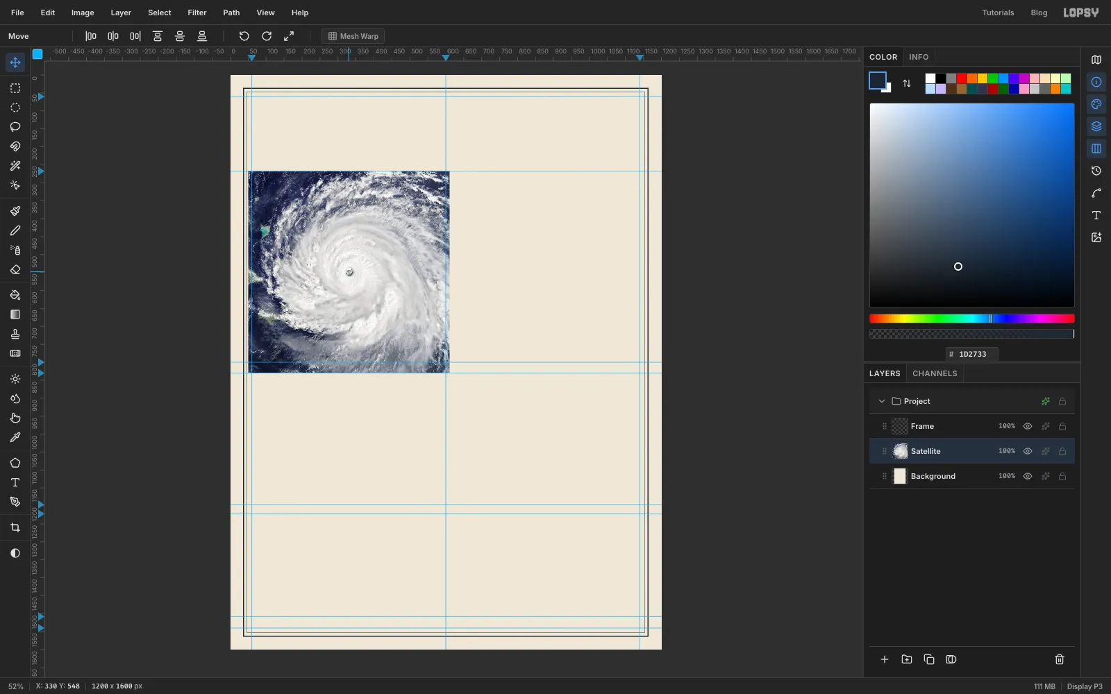
-
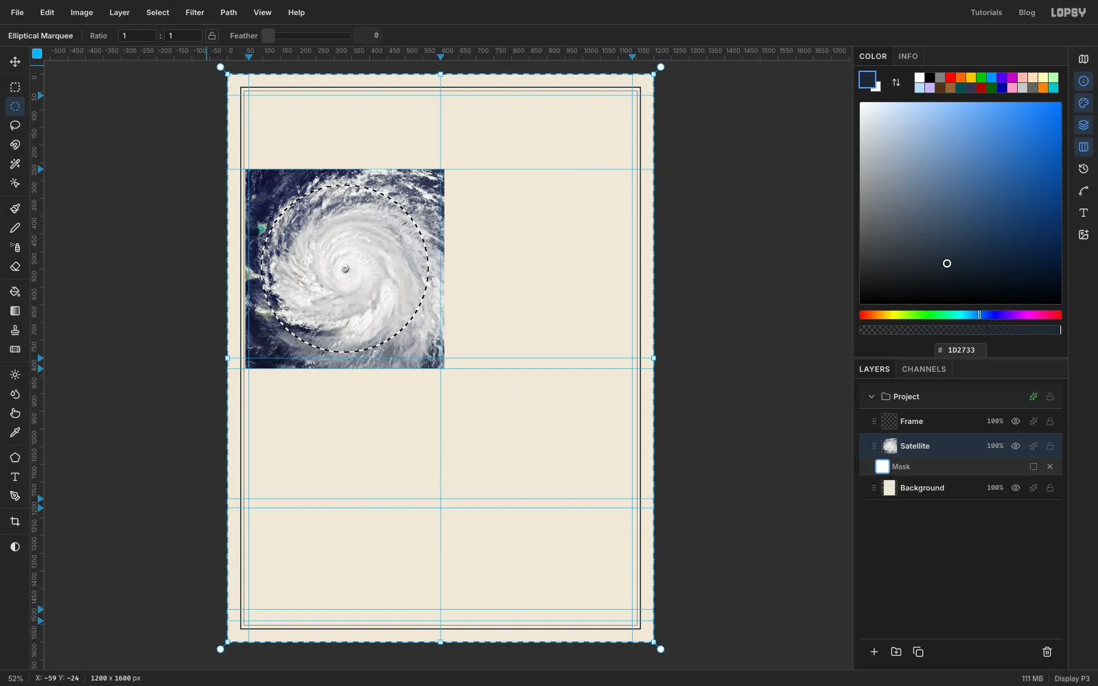
Mask the photo to a circle
- With Satellite selected, click Add Mask at the bottom of the Layers panel. A white mask appears under the layer.
- Click Edit mask for Satellite on the mask row. Now anything you fill goes into the mask, not the photo.
- Pick the Elliptical Marquee and make an exact-corner selection from
95, 313to565, 783. That's a 470 px circle around330, 548. - Choose Select → Inverse so everything outside the circle is selected.
- Set the foreground to black and choose Edit → Fill. Black in a mask hides, so the corners of the photo disappear.
- Deselect, and click the Satellite name to leave mask edit mode.
-
Turn the photo into a two-colour duotone
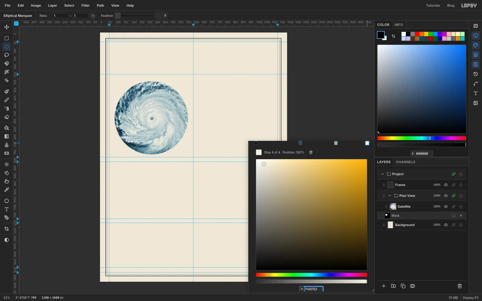
Old plates were printed in one or two inks, so the photo should look printed too. A Gradient Map replaces each brightness with a colour from a gradient. In Lopsy it lives on a group, so first put the photo in a group of its own:
- With Satellite selected, choose Layer → Group Layers and rename the new group
Plan View. - Click the ✦ (effects) button at the right of the group's row. The drawer that opens holds the group's adjustments. Click Add Adjustment → Gradient Map.
- Click the gradient bar at about 40% and again at about 72% to add two stops, so there are four.
- Click each stop in turn and type its colour into the hex field: at the dark end, , , and at the light end.
The ocean goes deep navy, the clouds go a soft blue-grey, and the brightest tops turn the colour of the paper. Close the drawer.
- With Satellite selected, choose Layer → Group Layers and rename the new group
-
Add a light halftone screen
A dot screen makes the photo feel printed rather than pasted in.
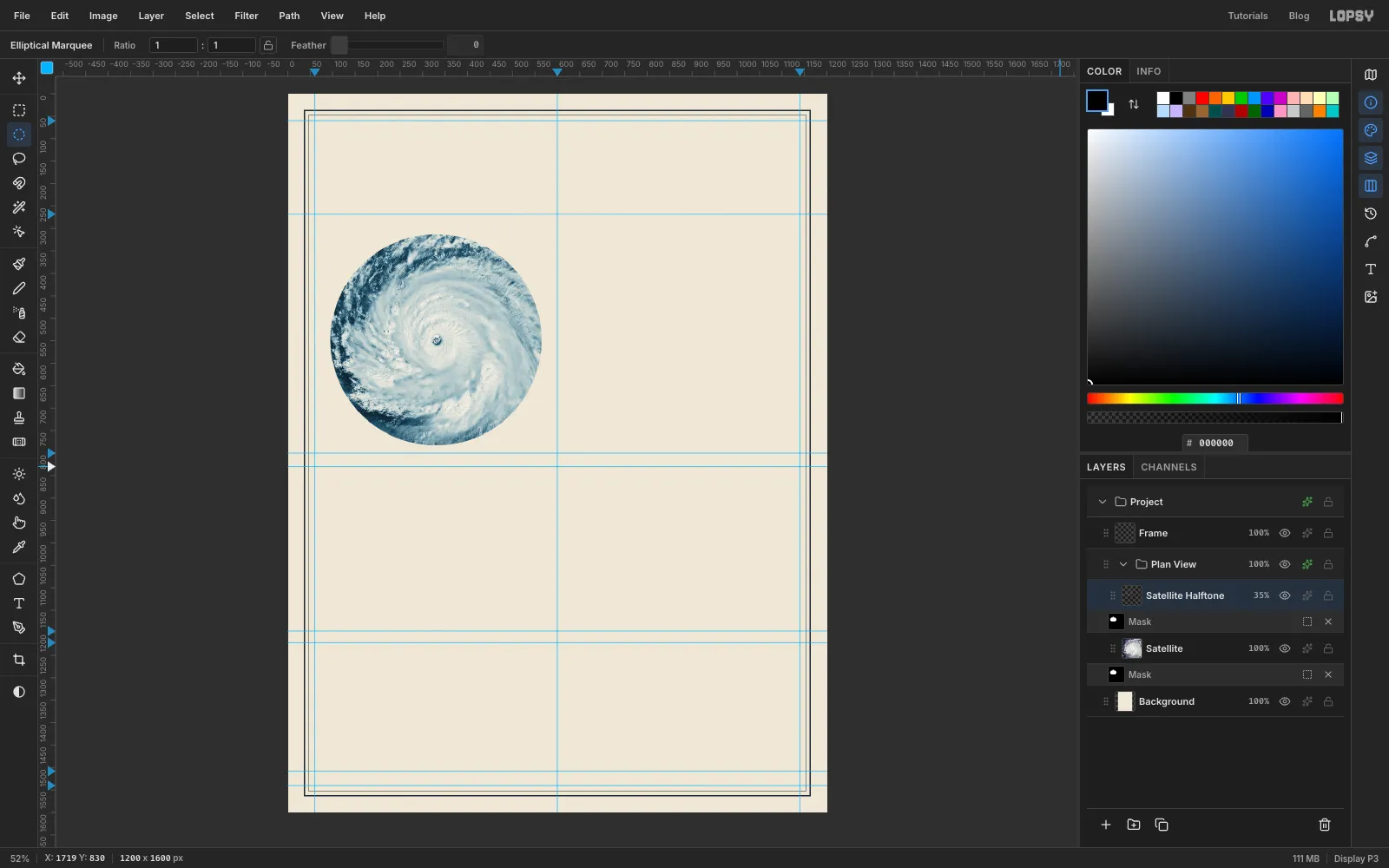
- Select Satellite and choose Layer → Duplicate Layer. Rename the copy
Satellite Halftone. It keeps the circle mask. - Choose Filter → Halftone… and set Dot Size to
4, Angle to45and Softness to1. Click Apply. - Open the layer's ✦ drawer, set the blend mode to Multiply, and close it.
- Set the layer's opacity to
35%with the percentage on its row.
The dots only darken, so the photo underneath still shows through, and the Gradient Map colours the dots navy as well.
- Select Satellite and choose Layer → Duplicate Layer. Rename the copy
-
Draw the wind-field rings
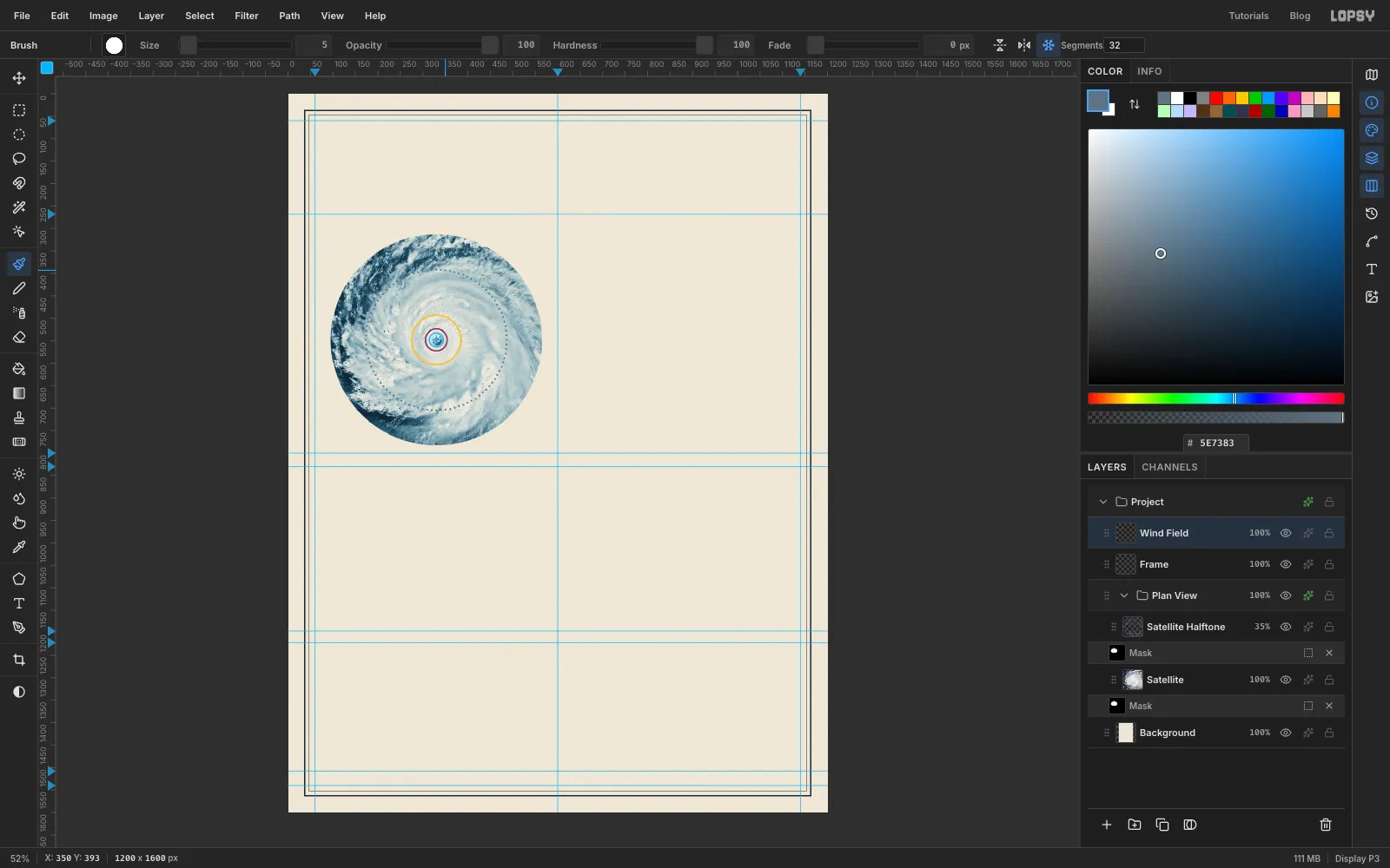
The rings show how far each wind speed reaches from the eye. On this disc, 1 km is about 0.52 px.
Click the Frame layer, click Add Layer, and name the new layer
Wind Field. Make each solid ring with Fill → Shrink → Delete, the biggest first, all centred on330, 548:- Hurricane-force winds, 110 km out: an exact-corner circle from
273, 491to387, 605, filled with yellow , shrunk by4, then Delete. - The Category 5 core, 50 km out: a circle from
304, 522to356, 574, filled with plum , shrunk by3, then Delete.
Tropical-storm winds reach 300 km out, which is 157 px. That one is a dotted ring in a quieter grey, so it doesn't compete with the other two:
- Pick the Brush (B) and set Size to
5and Hardness to100. Set the foreground to . - Turn on Radial Symmetry in the options bar and set its count to
32. - Hold Cmd and click the eye at
330, 548. That sets the centre of the symmetry. - Click once at
330, 391. You get 32 dots evenly spaced round the ring. - Click twice more just clockwise of the first dot, at about
340, 391and351, 392. That gives 96 dots in all, close enough to read as a dotted line.
Turn Radial Symmetry off. Then open the layer's ✦ drawer, tick Stroke, and set a 1 px ink stroke with the position outside. The thin outline keeps the yellow readable on the pale clouds.
- Hurricane-force winds, 110 km out: an exact-corner circle from
-
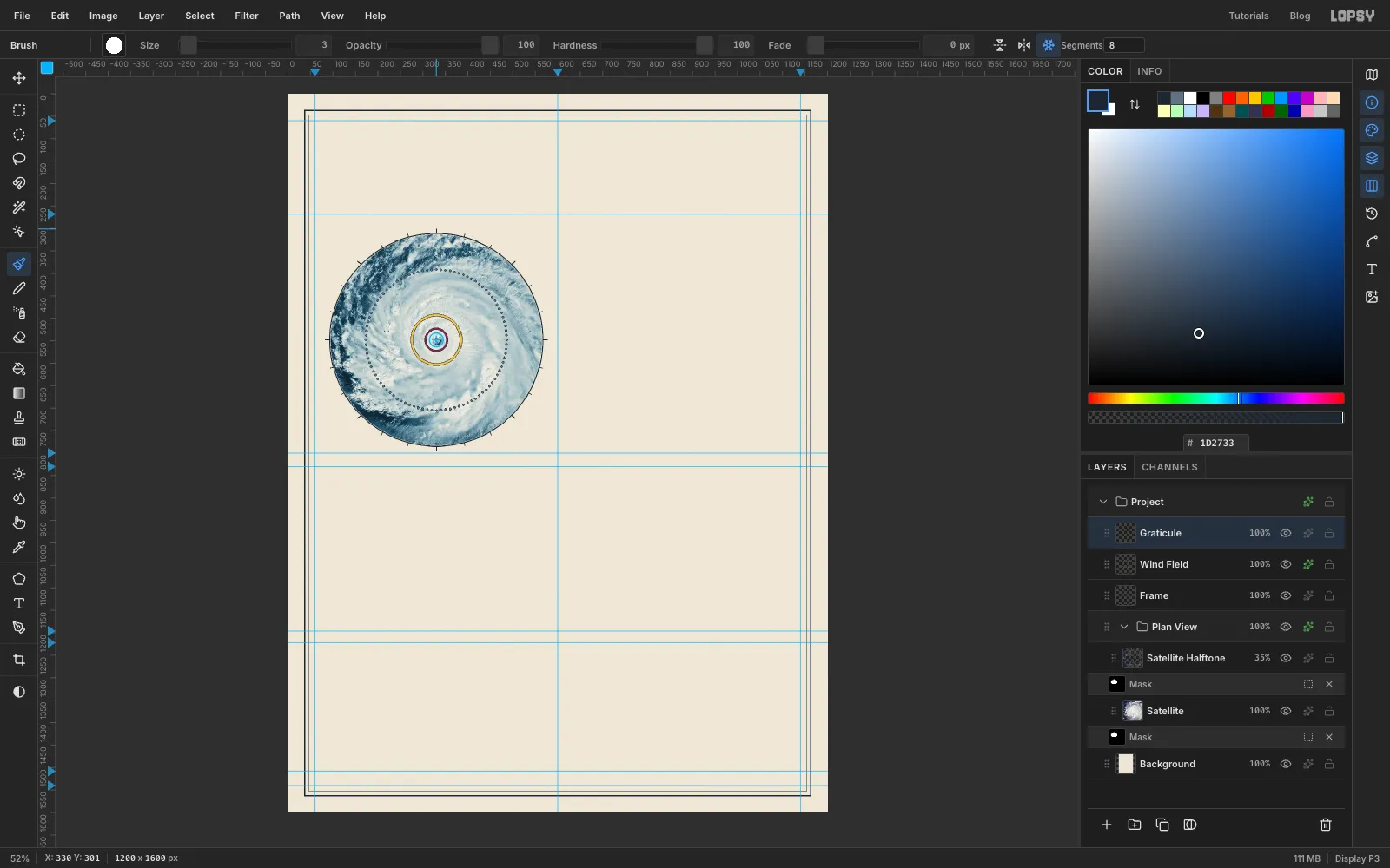
Add a rim and compass ticks
Add a layer called
Graticule.- Rim: select a circle from
92, 310to568, 786, just outside the photo. Fill it with ink, shrink by2, and press Delete. - Short ticks: pick the Brush with Size
2, turn Radial Symmetry on with a count of24, and Cmd-click the centre again. Click at330, 310, then Shift-click at330, 304. Shift-click draws a straight line from the last point, and the symmetry repeats it every 15°. - Long ticks: set the count to
8and the Size to3, Cmd-click the centre, then click at330, 310and Shift-click at330, 301. These land every 45°, on top of every third short tick.
- Rim: select a circle from
-
Draw a faint crosshair
Add a layer called
Crosshair. Set the symmetry count to4, the brush Size to1, and Cmd-click the centre. Click at330, 512and Shift-click at330, 315, just inside the rim. The four arms start 36 px from the eye, so they never cover it.Turn Radial Symmetry off and set the layer's opacity to
55%.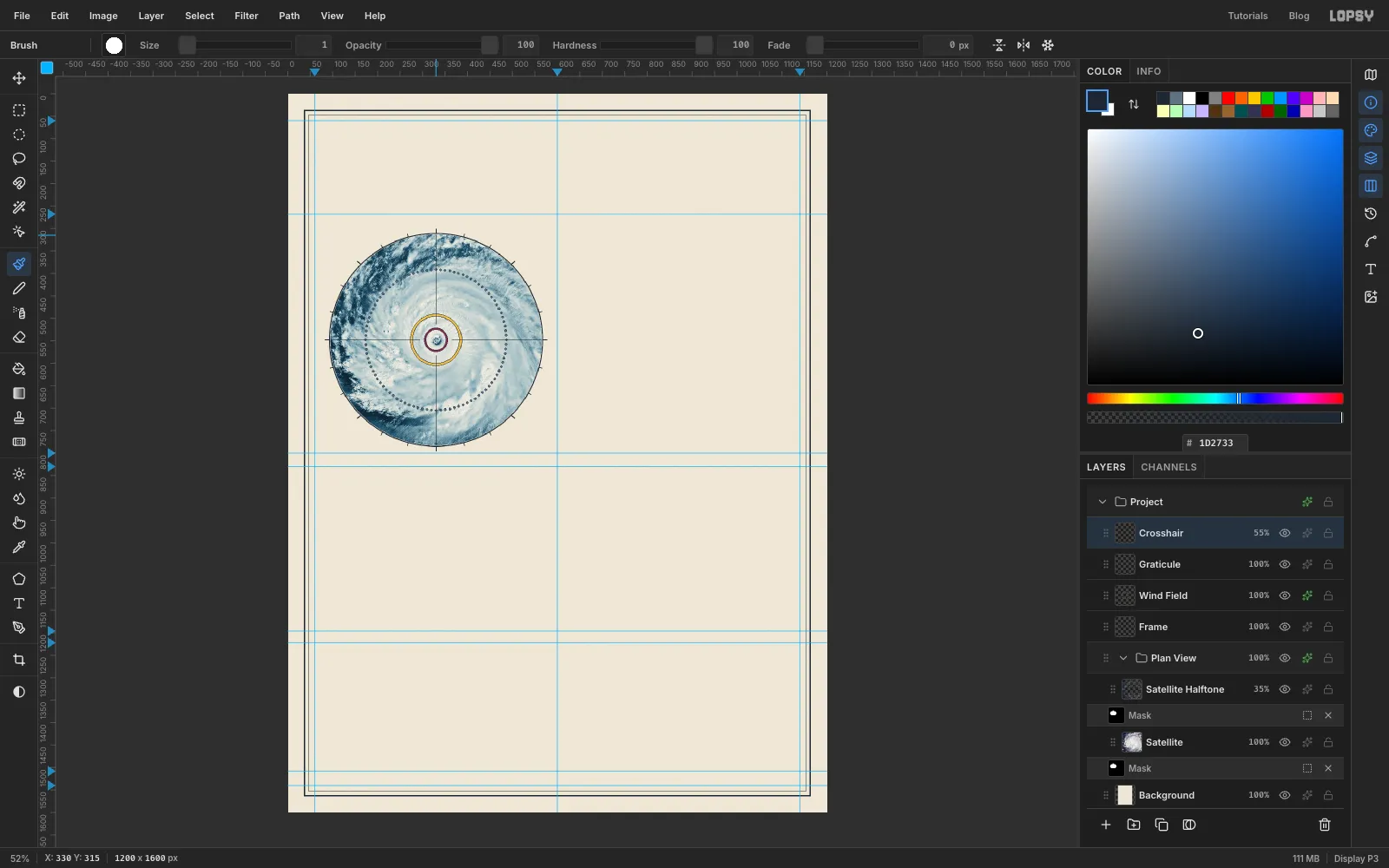
-
Lay the sea for the cross-section
Fig. 2 is drawn 8 px lower than its final spot, because at the end you'll nudge the whole figure up on the grid. Use the numbers as given.
Add a layer called
Seaand make an exact-corner selection from60, 1136to1140, 1166. Pick the Gradient tool, click Advanced… and set three stops: at the left end, at about 30%, and at the right end. Drag from the top of the selection straight down to the bottom. The thin orange line along the top stands for the warm surface water that feeds the storm.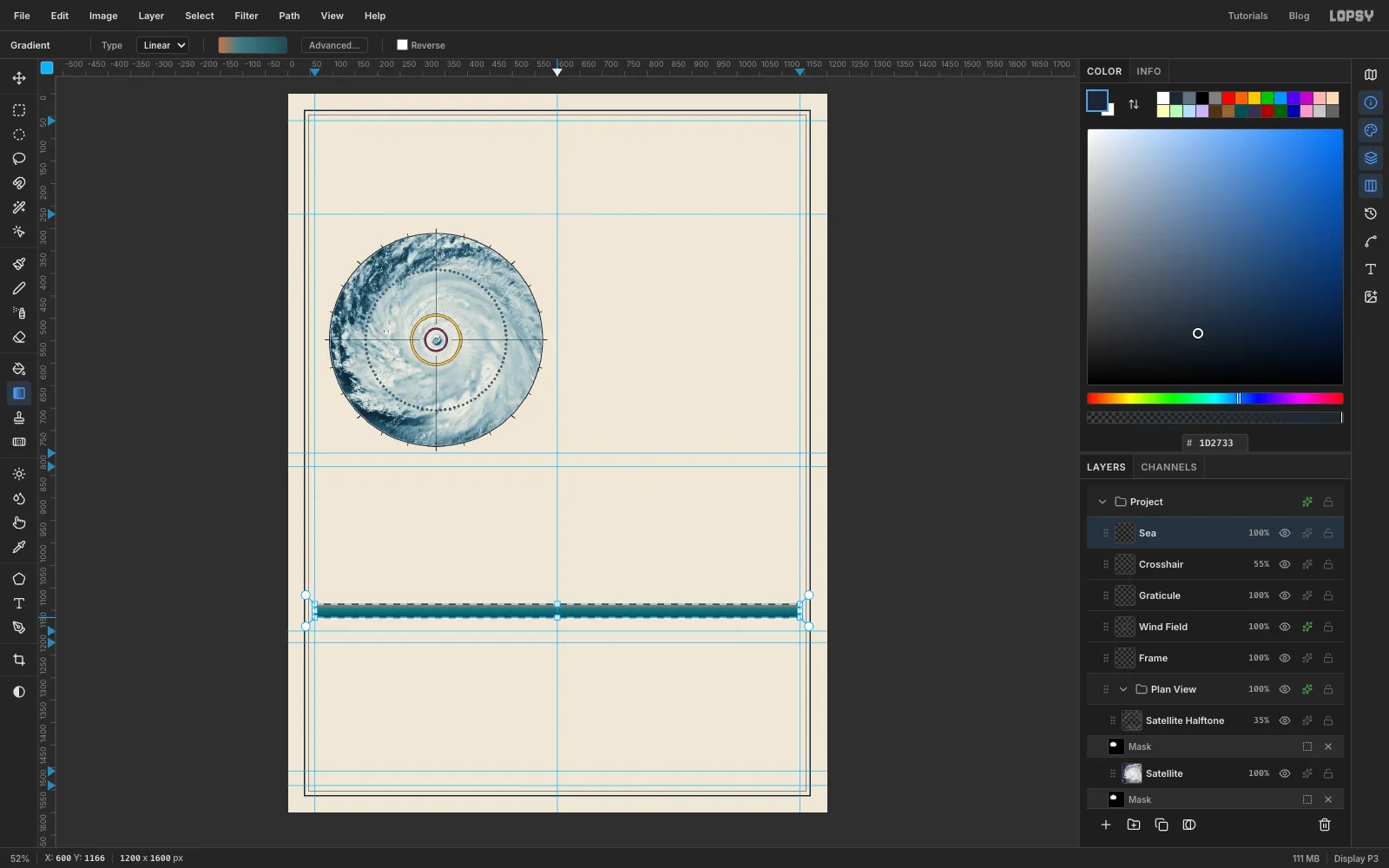
-
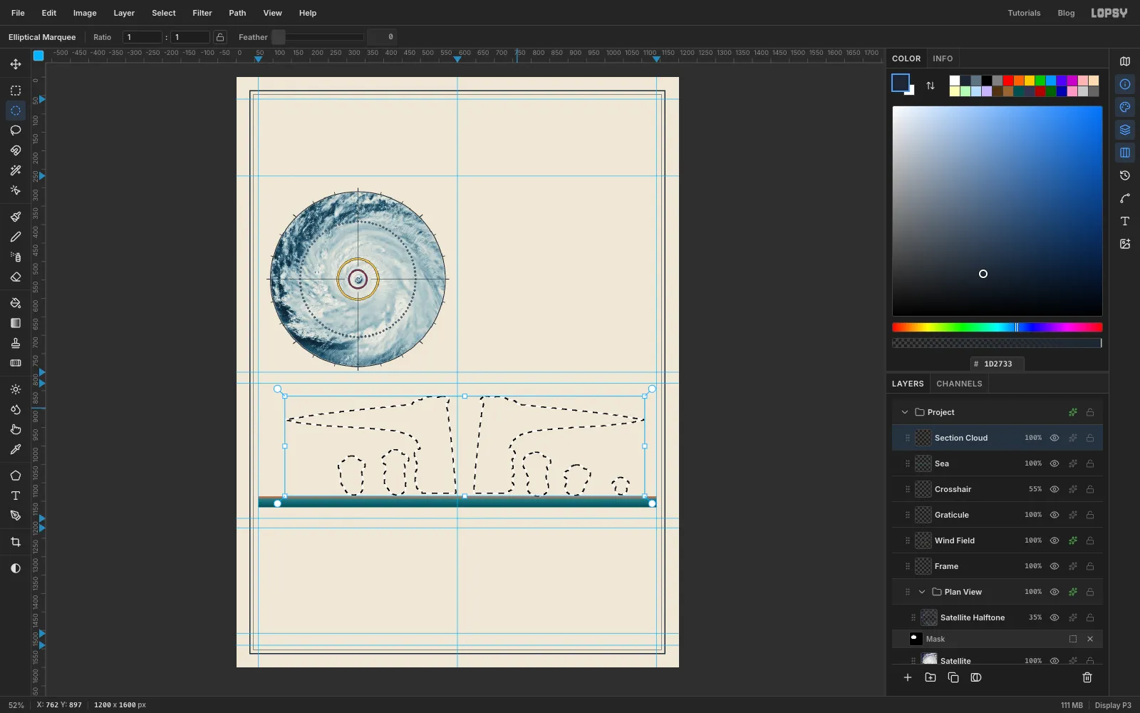
Build the cloud from shapes
The cross-section is drawn with a strong vertical stretch, about 15 times, so the storm doesn't look like a thin pancake. Each kilometre of height is 17 px, and sea level is at
y 1136, so 16 km is aty 864.Add a layer called
Section Cloud. The cloud is one big selection built from pieces:- Left half: pick the Lasso (L) and trace the left anvil and eyewall in one closed loop. Start at a thin point on the left at about
132, 929. Run along the top, rising gently to about540, 881beside the eye. Come down the eye side of the eyewall, slanting slightly inward, to596, 1127. Run left along the cloud base to504, 1127. Go up the outside of the eyewall, then curve out smoothly along the underside of the anvil and back to the tip. Smooth that inside corner: a sharp right angle there looks like a shelf. - Right half: hold Shift and trace the same shape flipped left to right around x
620, the middle of the eye. A point at x540on the left becomes x700on the right, so the right eyewall's inner wall starts at x644at the bottom. The gap between the two halves is the eye. It's narrow at the bottom and wider at the top. - Rainband towers: pick the Elliptical Marquee and Shift-drag overlapping ellipses to build cauliflower towers. Stack each one up from the cloud base like a pile of slightly wobbly cushions, and finish it with a cluster of three at the top. For the tallest left tower, between x
404and458: start with an ellipse about 54 px wide and 46 px tall centred at431, 1111, just above the base. Add four more of about the same size, each about 20 px higher and a few pixels left or right of the one below. Then add three smaller ones round the top, the highest reaching abouty 1010. I made five towers: two on the left, reaching about 6 and 7 km, and three on the right, at about 7, 5 and 3 km. Keep them below the anvil. - Lumpy edges: add a few more Shift ellipses down the outside of each eyewall, and two or three bumps at the top of each eyewall for the overshooting storm tops.
- Left half: pick the Lasso (L) and trace the left anvil and eyewall in one closed loop. Start at a thin point on the left at about
-
Flatten the cloud bases
Real cumulus clouds have flat bottoms where the air reaches the height at which it condenses. Pick the Rectangular Marquee, hold Alt, and drag a rectangle from just above the sea at about
70, 1128down past the sea's bottom edge. Alt subtracts it, so every tower now ends in a straight line half a kilometre above the water.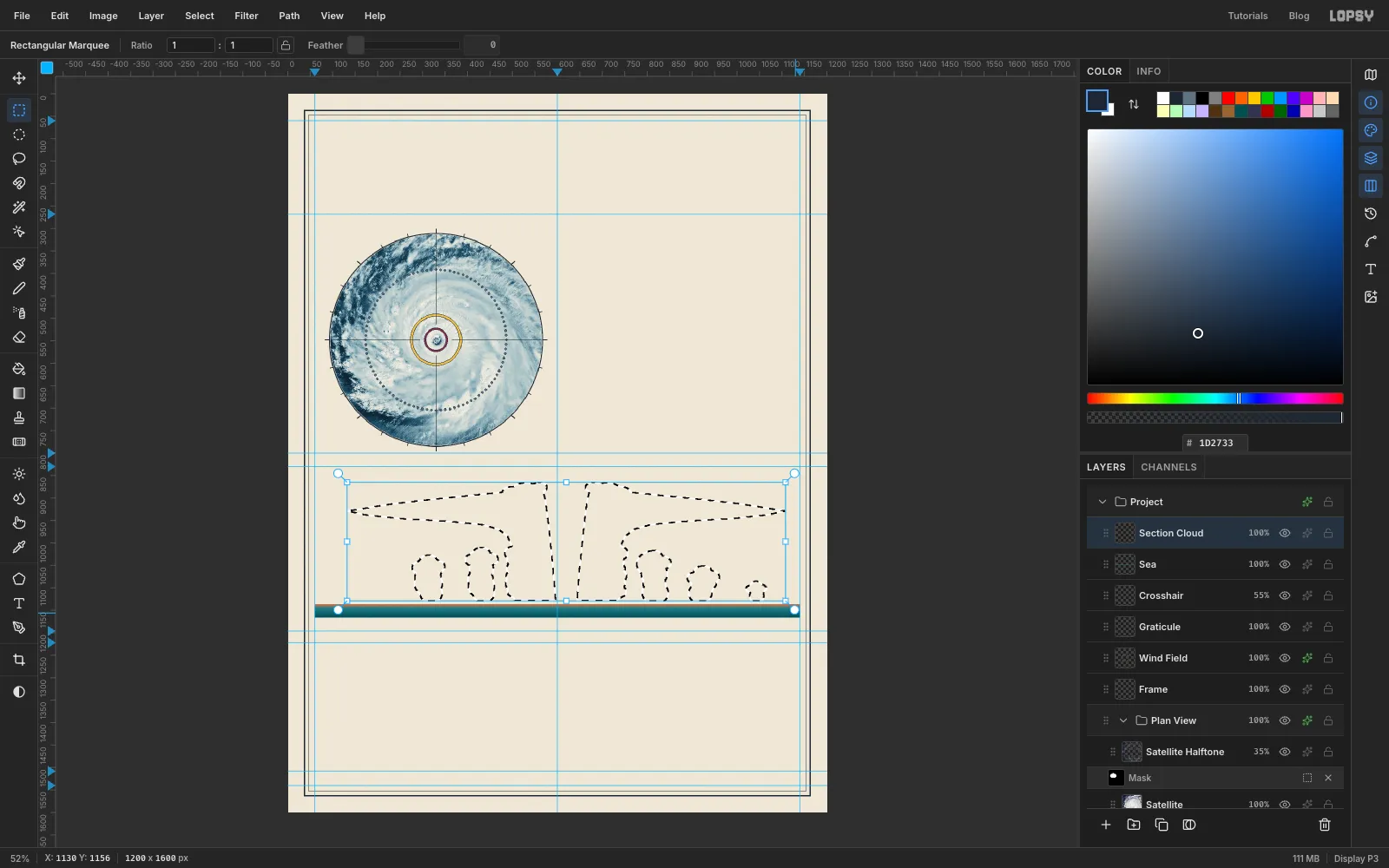
-
Fill the cloud and outline it
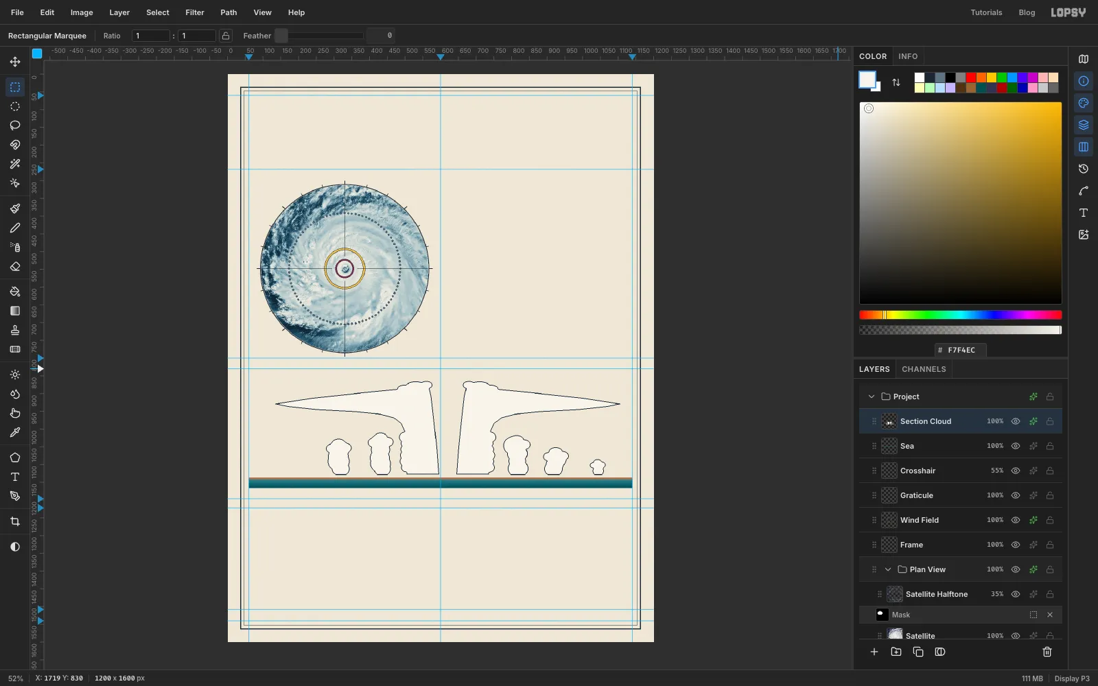
Set the foreground to and choose Edit → Fill, then deselect. Open the layer's ✦ drawer, tick Stroke, and set a 2 px ink stroke with the position inside. An inside stroke keeps the outline crisp right against the paper.
-
Make a hatch tile and load the cloud's shape
Engravers shaded with lines, not soft blurs. First make a hatch tile to paint with:
- Add a temporary layer. Pick the Pencil (N) at Size
1with the foreground set to rule blue . In the empty strip under the frame, click at1168, 1575and Shift-click at1175, 1568. That's a diagonal across an 8 px square. - Select exactly that square, from
1168, 1568to1176, 1576, and choose Edit → Define Pattern. - Deselect, then delete the temporary layer with the bin button at the bottom of the Layers panel.
Now work out where the shading goes. With the light coming from the top left, it belongs on the lower right edge of each cloud:
- Click Section Cloud, then Add Layer, and name the new layer
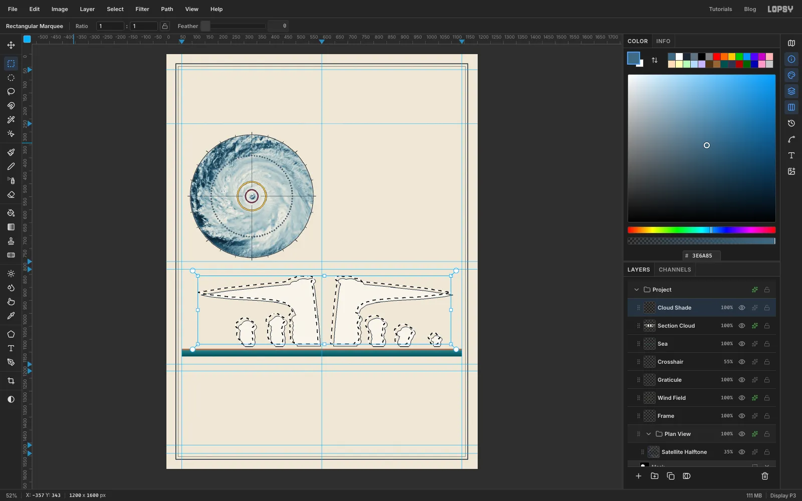
Cloud Shade. - Cmd-click the Section Cloud thumbnail to select the cloud's shape.
- With the Rectangular Marquee active, press Shift+Left and then Shift+Up. That moves the selection outline 10 px up and to the left, without moving any pixels.
- Add a temporary layer. Pick the Pencil (N) at Size
-
Select a shading band
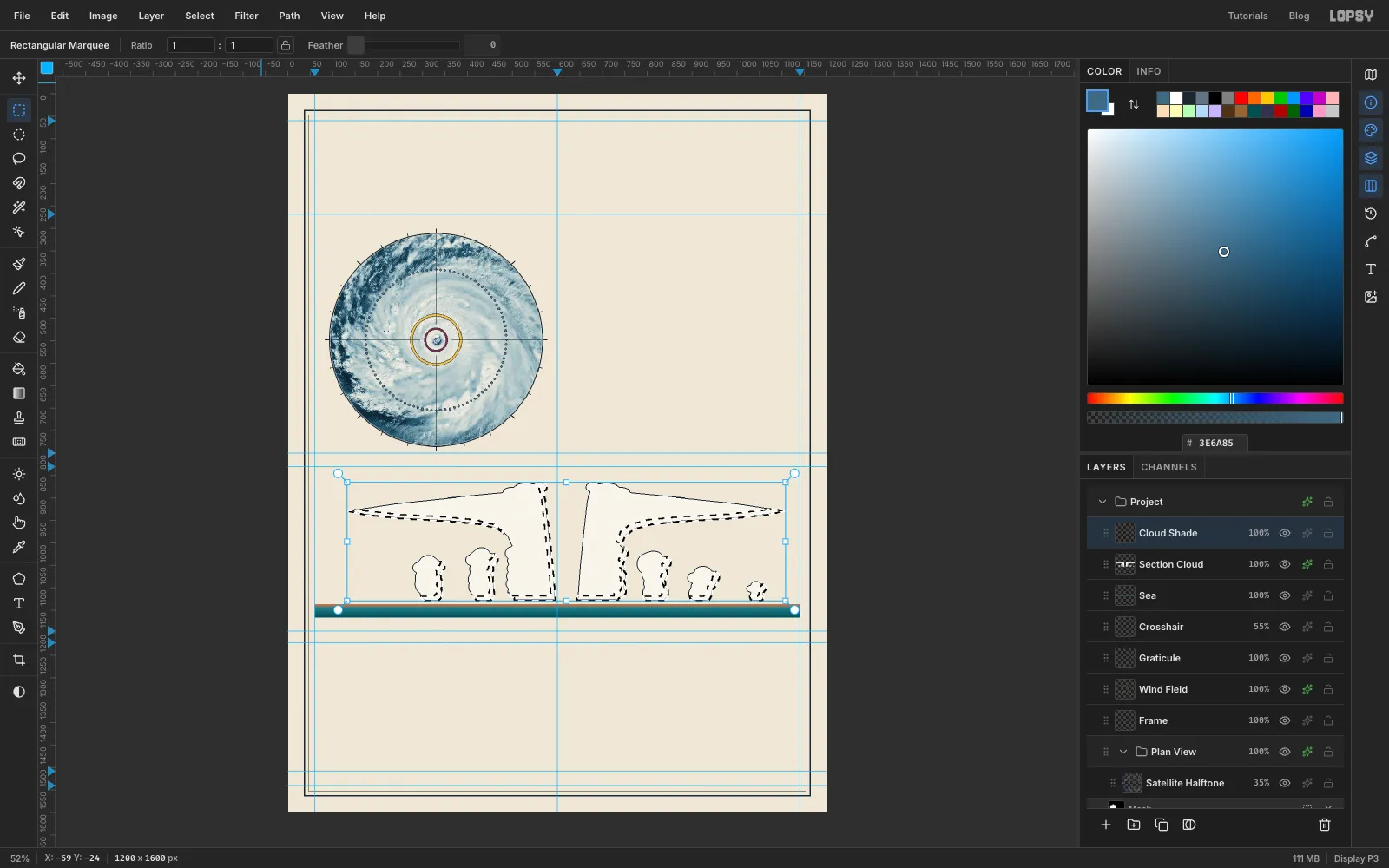
- Choose Select → Inverse. Everything except the shifted cloud is now selected.
- Hold Cmd, Shift and Alt together and click the Section Cloud thumbnail again. That intersects the selection with the real cloud, so you're left with a 10 px band along the lower right of every cloud.
-
Fill the band with hatching
Choose Edit → Fill with Pattern…, pick the diagonal tile you just defined, and click Apply. Deselect and set the layer's opacity to
75%. The hatching gives the clouds volume and looks drawn rather than airbrushed.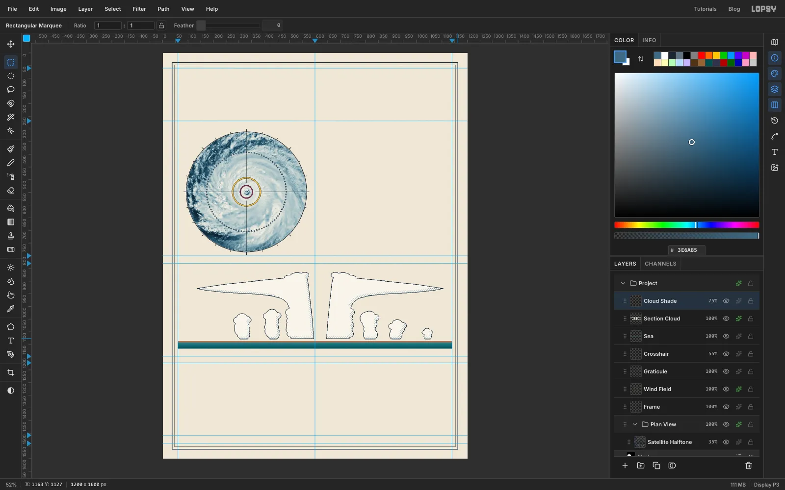
-
Add the height axis, scale bar and tropopause
Add a layer called
Section Axis. Pick the Pencil at Size1with ink as the foreground.- Axis: click at
104, 1136and Shift-click at104, 864. - Ticks: draw one every 17 px, the same way, pointing left from the axis toward where the numbers will go. Make them 6 px long, and 12 px long at 0, 5, 10 and 15 km.
- Scale bar: the section's horizontal scale is about 1.1 px per km, so 100 km is 111 px. Fill a 3 px bar from
975to1086at abouty 997, and draw a short tick at each end.
Add a layer called
Tropopause. That's the ceiling where the storm's clouds stop rising. Pick the Brush at Size3. Click the brush tip swatch at the left end of the options bar to open the Brushes panel, and on its Shape tab set Spacing to300%. Each dab now lands well apart from the last, which gives a dotted line. With rule blue as the foreground, click at116, 864and Shift-click at1128, 864. Then switch to ink and draw the sinking air down the eye, from621, 908to621, 1102. Set Spacing back to1%when you're done.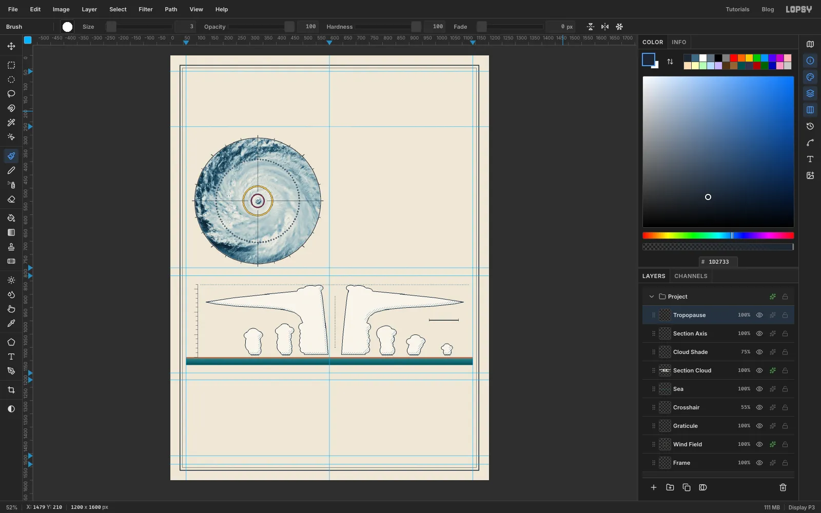
- Axis: click at
-
Draw the airflow with the Pen
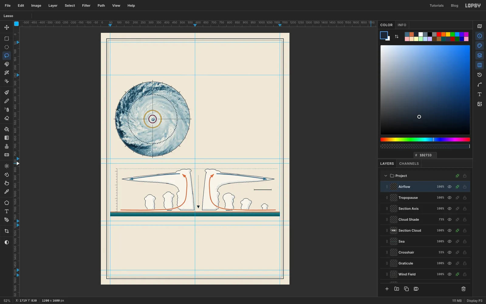
This is the heart of the plate: one loop of air. It comes in warm and moist over the sea, rises up the eyewall, and spreads out as cold cirrus at the top.
Add a layer called
Airflow. Pick the Pen tool (P) and set Stroke to5.- Warm air in and up: set the foreground to . Click at
128, 1126to start. At each of the next points, press and drag a short way, about 20–40 px, in the direction the air is travelling. That pulls out handles that keep the curve smooth through the point. The points are: along the sea at330, 1126, rising at466, 1116, curving up into the eyewall at532, 1075, straight up at548, 983, and turning left at544, 925. Finish with a plain click at522, 900. Press Enter to stroke the path with the foreground colour, then delete the path in the Paths panel. - Cold air out: in rule blue, draw a second path the same way: click at
502, 896, drag through420, 900and290, 915, and click at186, 930. Stroke it and delete the path. - The right side: draw both paths again as mirror images. To get each point, subtract its x from
1240and keep the y, so128, 1126becomes1112, 1126.
For arrowheads, pick the Lasso and drag a small triangle at the end of each path in three straight strokes, about 20 px long and 18 px across the base, pointing the way the path ends. Fill it in that path's colour. Add an ink one pointing down at the bottom of the dotted line in the eye.
Finish with a 2 px Stroke effect in , position outside. The pale halo lifts the arrows off the cloud outlines where they cross.
- Warm air in and up: set the foreground to . Click at
-
Rule the chart grids
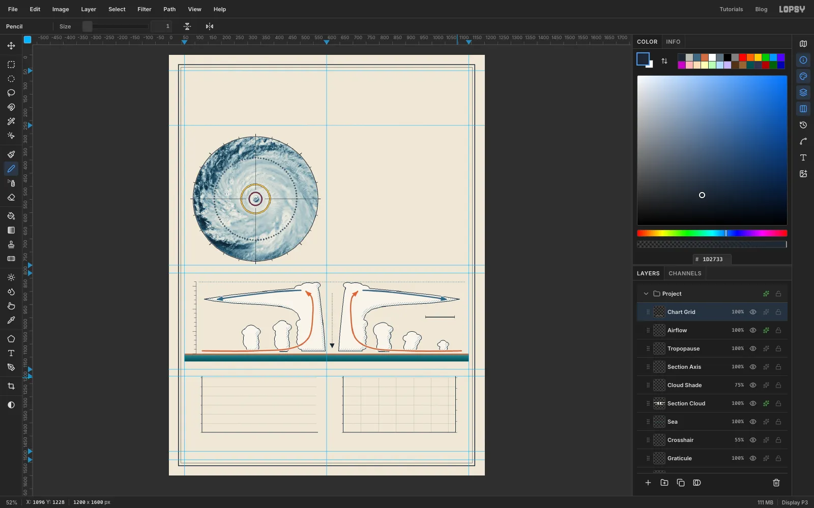
Add a layer called
Chart Grid. Both plots run fromy 1228at the top toy 1436at the bottom.- Hairlines: pick the Pencil at Size
1in . For Fig. 3 (x128–560), draw a horizontal line every 50 km/h. Each 50 km/h is about 35 px. Fig. 4 runs from x664to1090and gets the same horizontals, plus a vertical line every 50 km. Each 50 km is about 67 px, so 300 km lands at x1063, with a little room left before the pressure axis at x1090. - Axes: switch to ink at Size
2. Fig. 3 gets a left axis and a baseline. Fig. 4 gets a left axis for wind, a baseline and a right axis for pressure. - Ticks: add 6 px ink ticks at Size
1beside each axis.
- Hairlines: pick the Pencil at Size
-
Draw the Saffir–Simpson bars
Add a layer called
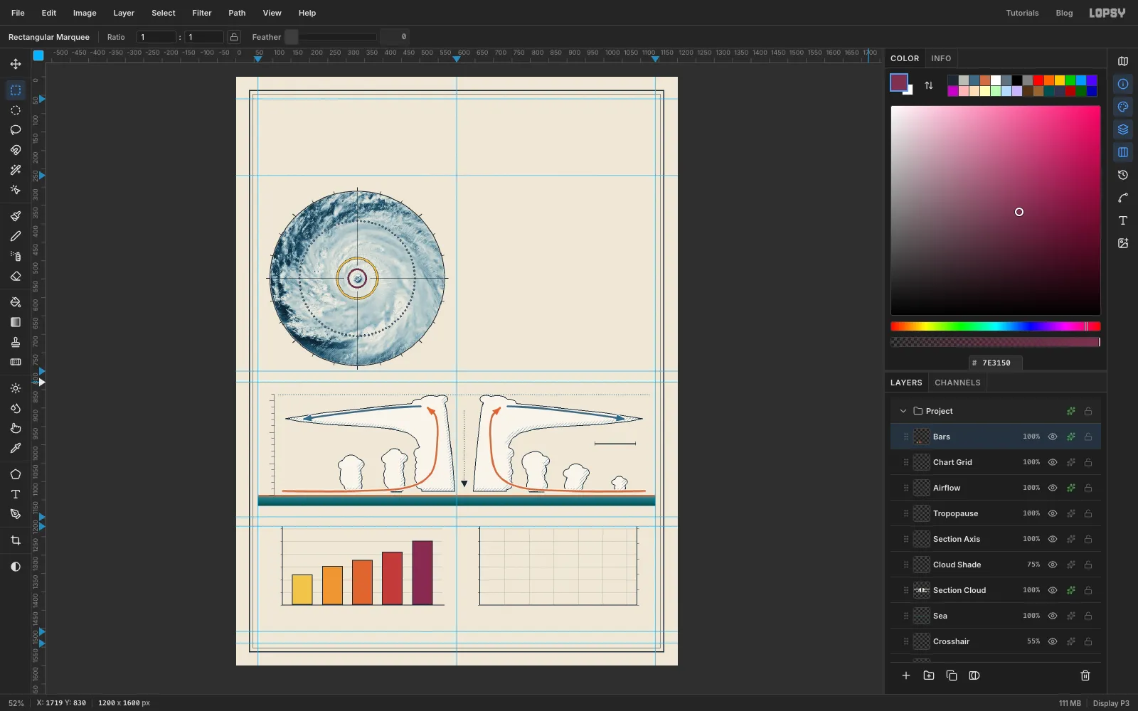
Bars. Each bar is 56 px wide with about 25 px between them, and its height is the category's minimum wind speed on the 0–300 km/h scale. All five run down to the baseline aty 1436:- CAT 1, 119 km/h: from
153, 1354, in yellow - CAT 2, 154 km/h: from
235, 1329, in orange - CAT 3, 178 km/h: from
316, 1313, in red-orange - CAT 4, 209 km/h: from
397, 1291, in red - CAT 5, 252 km/h: from
479, 1261, in plum
Make each bar with an exact-corner rectangle down to the baseline and Edit → Fill it in its colour. Then give the layer a 2 px ink Stroke, position inside.
These are the same colours used in Fig. 1: yellow is the hurricane-force ring and plum is the Cat 5 core. Keeping colours consistent across figures is what makes a plate read as one piece.
- CAT 1, 119 km/h: from
-
Plot wind and pressure
- Eyewall band: add a layer called
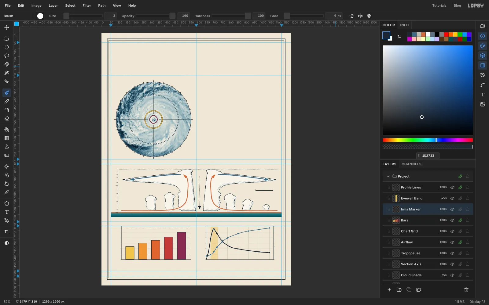
Eyewall Band. Fill a rectangle from 20 km to 55 km out (x691–737), the full height of the plot, in yellow, and set the layer to45%. That's where the fastest winds are. - Curves: add a layer called
Profile Lines. The left axis is wind, 0 to 300 km/h, and the right axis is pressure, 910 hPa at the baseline up to 1010 at the top. Here are the data points, as distance from the eye:
- Pressure, hPa: 0 km 921, 20 km 925, 36 km 934, 50 km 948, 75 km 964, 100 km 976, 150 km 989, 200 km 997, 250 km 1002, 300 km 1006
- Wind, km/h: 0 km 0, 10 km 70, 20 km 190, 30 km 268, 36 km 280, 50 km 240, 75 km 170, 110 km 119, 150 km 98, 200 km 82, 250 km 71, 300 km 63
With the Pen, click the first point, press-and-drag through the middle ones, and click the last, as you did for the arrows. Stroke the pressure curve in rule blue at Stroke
3and the wind curve in ink at Stroke4. The wind passes 119 at 110 km and 63 at 300 km, which match the yellow ring and the dotted ring in Fig. 1, so the figures agree. Ink rather than red keeps red meaning Category 4 only.- Data dots: pick the Brush at Size
9and click once on every data point, in each curve's colour. Give the layer a 2 px paper-coloured Stroke outside, so the dots stand off the lines. - Irma's peak: click Bars, add a layer called
Irma Marker, and draw a dotted ink line across Fig. 3 at 280 km/h, using the 300% spacing trick again.
- Eyewall band: add a layer called
-
Add rules, leaders and the Cat 5 stamp
- Rules: on the Frame layer, fill a 4 px ink rule across the page at
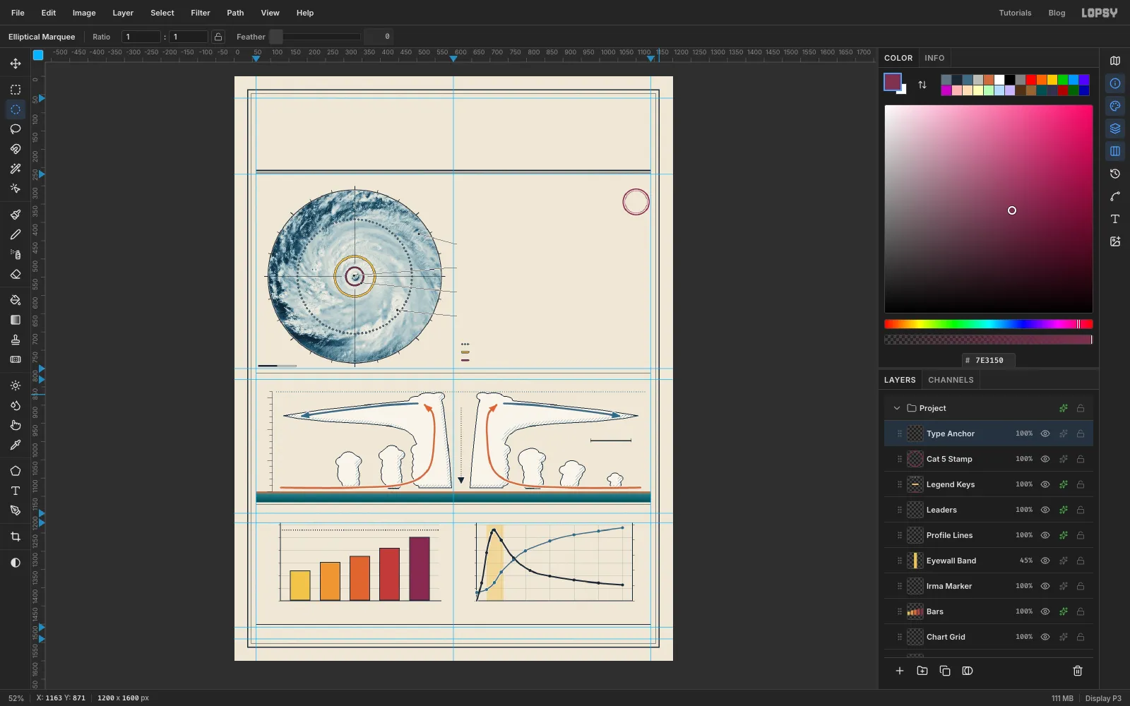
y 256and a 1 px rule aty 264, for a classic heavy-and-light header rule. Add 1 px dividers aty 813,1172and1500. - Leaders: add a layer called
Leaders. With the Pencil at Size1, click on a feature, Shift-click atx 600on its callout row, then Shift-click atx 610. The four leaders are:
- cirrus at the top right, from
505, 432to the row aty 458 - the eye, from
328, 546toy 524 - the eyewall, from
348, 566on the plum ring toy 590 - a rainband at the lower right, from
446, 640toy 656
Click a 7 px Brush dot on each feature end. Keep the eye and eyewall ends well apart, or the two leaders read as one. A 1 px paper Stroke outside keeps the leaders visible over the clouds.
- Scale bar: on the same layer, fill an ink bar from
66, 790to170, 795. That's 104 px, or 200 km at this scale. Then fill118, 791to169, 794with paper colour , leaving a thin ink border round the right half. That gives the classic two-block bar. - Legend keys: add a layer called
Legend Keyswith three grey brush dots, a short yellow bar and a short plum bar, stacked down the right column atx 622. Give the layer a 1 px ink Stroke. - Stamp: add a layer called
Cat 5 Stampand make two plum rings around1100, 344, one of radius 37 shrunk by3and one of radius 31 shrunk by1.
- Rules: on the Frame layer, fill a 4 px ink rule across the page at
-
Label the charts
Before typing anything, add one empty layer at the top called
Type Anchor, and click it before every new piece of text. When a text layer is selected, the Text options restyle that layer, so starting each new label from an ordinary layer keeps the last one safe.Work from the bottom of the page upward. A click with the Text tool (T) inside an existing text line's box edits that text instead of starting a new one, and the box reaches below and to the right of the words. Building upward means you never click into a line you've already set.
Three typefaces do all the work: Barlow Condensed for titles, IBM Plex Mono for data, and Instrument Serif for prose. Check each label's Letter spacing in the Text panel as you go. It's
0unless a step says otherwise, and the last value carries over to the next new text. Rename each text layer after its job, such asTitle,Fig 3 HeadorAlt 5.Within each list below, the items run from the bottom of the page up, so you can type them in that order.
- Footer: at
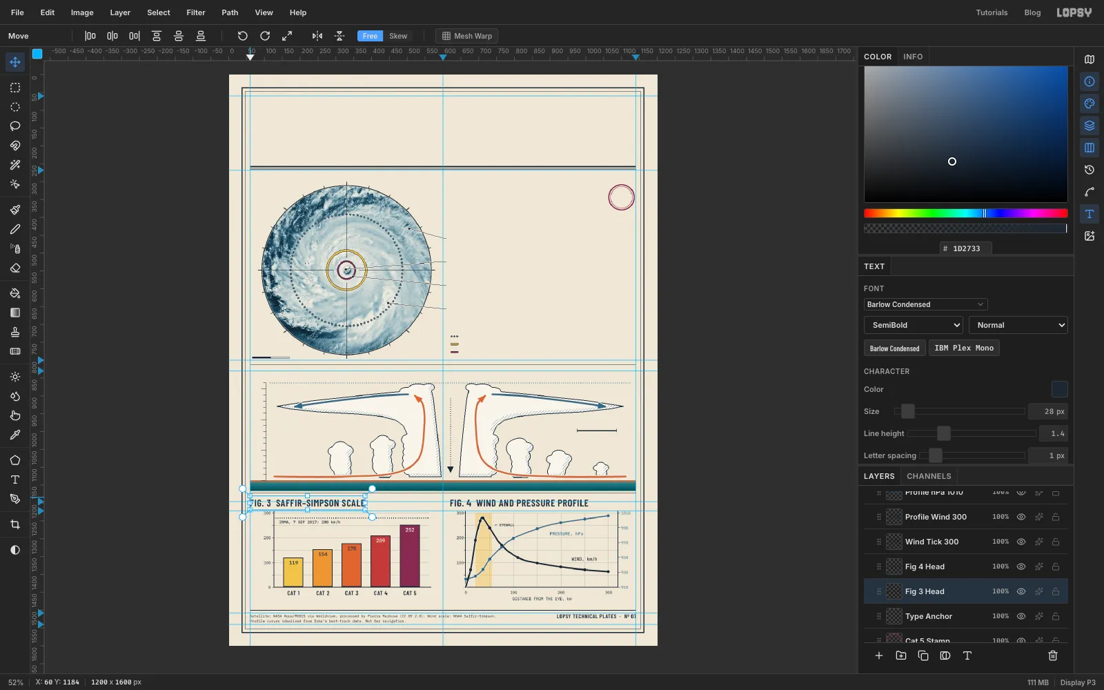
y 1512, a two-line source note in Plex Mono at10px: "Satellite: NASA Aqua/MODIS via Worldview, processed by Pierre Markuse (CC BY 2.0). Wind scale: NOAA Saffir–Simpson." and "Profile curves idealised from Irma’s best-track data. Not for navigation." On the right, "LOPSY TECHNICAL PLATES · Nº 07" in Barlow Condensed SemiBold at16px, right-aligned to the margin. - Axis numbers: Plex Mono at
11px. Wind numbers and distances are ink, and pressure numbers are blue. Fig. 4 shares the0on its distance axis, so leave the wind axis's0off. Add "DISTANCE FROM THE EYE, km" under Fig. 4. - Bars: values in Plex Mono Medium at
14px, sitting 9 px inside each bar's top edge. They're ink on the three lighter bars and paper-coloured on the two darker ones, so each has enough contrast. Category names go underneath in Barlow Condensed SemiBold at17px. - Series: "WIND, km/h" above the ink curve, "PRESSURE, hPa" below the blue one, and a small "← EYEWALL" just right of the yellow band.
- Irma's peak: "IRMA, 7 SEP 2017: 280 km/h" in Plex Mono Medium at
11px, just under the dotted line in Fig. 3 and about 14 px in from the axis. - Titles: "FIG. 3 SAFFIR–SIMPSON SCALE" and "FIG. 4 WIND AND PRESSURE PROFILE" in Barlow Condensed SemiBold at
28px with1px letter spacing.
- Footer: at
-
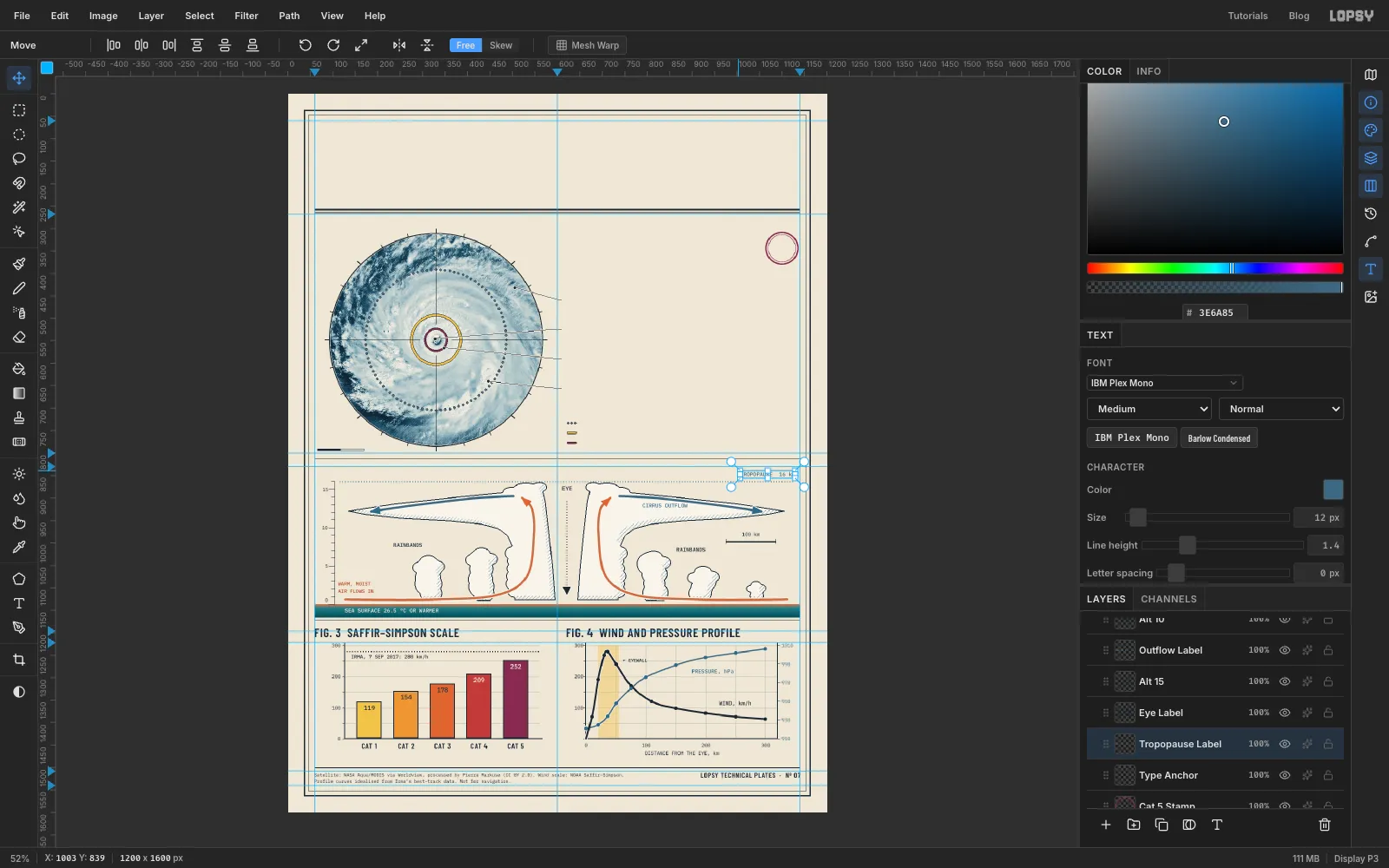
Label the cross-section
Keep going upward, still in Plex Mono Medium at
11–12px unless noted:- "SEA SURFACE 26.5 °C OR WARMER" in paper colour on the teal band, starting at
x 128. That's the minimum water temperature a hurricane needs. 0beside the bottom tick, lifted a few pixels so it doesn't touch the orange surface line.- "WARM, MOIST / AIR FLOWS IN" on two lines in dark orange , starting at
x 112just above the incoming arrow. It labels the air, not the water. 5and10beside their long ticks, right-aligned tox 88.- "RAINBANDS" twice: over the two left towers, and beside the right towers just left of the scale bar. Put "100 km" over the scale bar.
- "CIRRUS OUTFLOW" in rule blue inside the right anvil, under its arrow.
- "EYE" in ink at
13px, centred in the gap between the overshooting tops, and15beside the top long tick. - One line along the top, just above the dotted tropopause:
- "FIG. 2 CROSS-SECTION THROUGH THE EYE" in Barlow Condensed SemiBold at
28px. - "VERTICAL SCALE EXAGGERATED ABOUT 15×" in Plex Mono at
12px. - "TROPOPAUSE 16 km" in rule blue, right-aligned.
Type them right to left. The title sits above the plot, like the other three.
- "SEA SURFACE 26.5 °C OR WARMER" in paper colour on the teal band, starting at
-
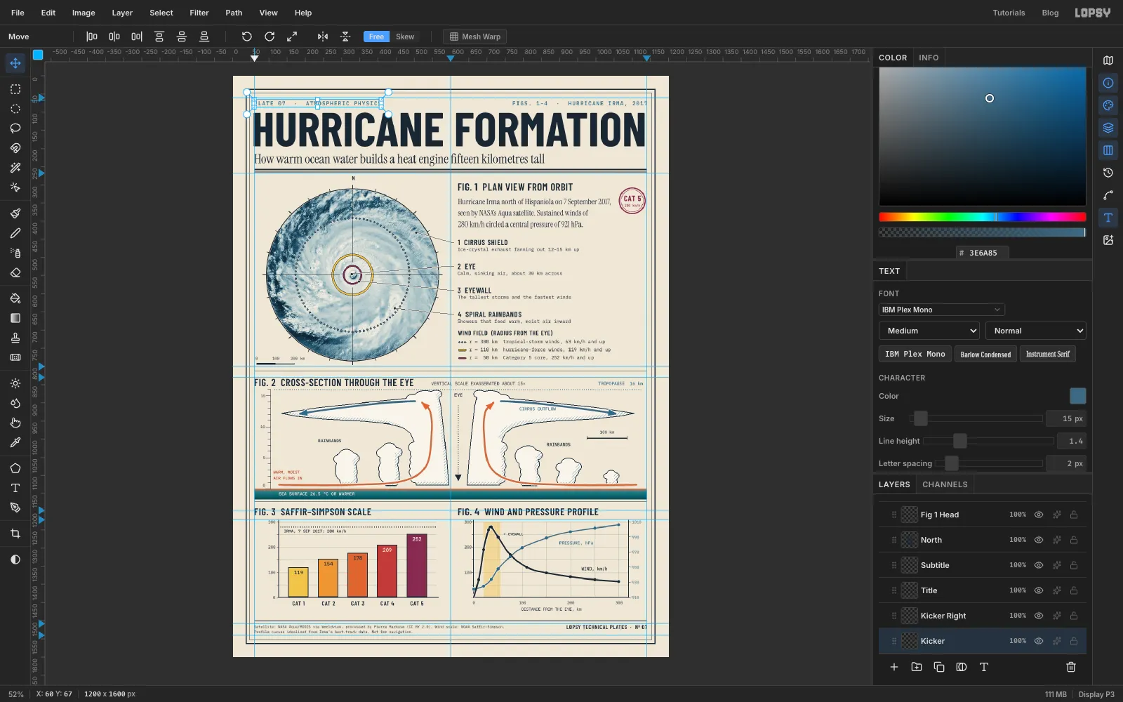
Set the headline and the Fig. 1 text
- Scale bar labels:
0,100and200 kmin Plex Mono at11px over the bar under the disc. - Legend rows: in Plex Mono at
13px, starting atx 652beside the keys: - "r = 300 km tropical-storm winds, 63 km/h and up"
- "r = 110 km hurricane-force winds, 119 km/h and up"
- "r = 50 km Category 5 core, 252 km/h and up"
- Legend title: "WIND FIELD (RADIUS FROM THE EYE)" in Barlow Condensed SemiBold at
18px, aty 700. - Callouts: four titles in Barlow Condensed SemiBold at
21px, each centred on its leader row (y 656,590,524and458). Each has a note in Plex Mono at13px just under it. Type the note first, then the title above it: - "4 SPIRAL RAINBANDS": "Showers that feed warm, moist air inward"
- "3 EYEWALL": "The tallest storms and the fastest winds"
- "2 EYE": "Calm, sinking air, about 30 km across"
- "1 CIRRUS SHIELD": "Ice-crystal exhaust fanning out 12–15 km up"
- Stamp: "280 km/h" in tiny plum Plex Mono, with "CAT 5" in plum Barlow Condensed Bold above it, centred in the rings.
- Fig. 1 caption: at
x 620, y 338, in Instrument Serif at22px, on three lines: "Hurricane Irma north of Hispaniola on 7 September 2017, / seen by NASA’s Aqua satellite. Sustained winds of / 280 km/h circled a central pressure of 921 hPa." - Fig. 1 title: "FIG. 1 PLAN VIEW FROM ORBIT" in Barlow Condensed SemiBold at
28px. - North: a small "N" over the top tick.
- Deck: "How warm ocean water builds a heat engine fifteen kilometres tall" in Instrument Serif at
36px, just above the header rule. - Headline: "HURRICANE FORMATION" in Barlow Condensed Bold at
132px with0letter spacing. It fills the measure from margin to margin. - Kickers: "PLATE 07 · ATMOSPHERIC PHYSICS" top left and "FIGS. 1–4 · HURRICANE IRMA, 2017" top right, in Plex Mono Medium at
15px with2px letter spacing, in rule blue.
- Scale bar labels:
-
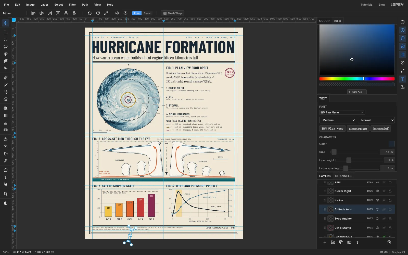
Turn the axis titles on their side
The two charts that measure height and speed need a vertical axis title.
- Click Type Anchor and type "ALTITUDE, km" in Plex Mono Medium at
11px, in the empty strip below the frame. - Switch to the Move tool. Live text has its own handles. Hold Cmd and drag the round rotate handle at its top right corner a quarter turn anticlockwise. Cmd snaps the angle to 15° steps, so stop when it reads −90°. If it lands one step short, press Cmd+Z and drag a little further.
- Drag it with the Move tool up beside the Fig. 2 axis, then use the arrow keys to centre it between the frame and the altitude numbers.
Do the same with "MIN. SUSTAINED WIND, km/h" for Fig. 3. The text stays live, so you can still fix a typo later.
- Click Type Anchor and type "ALTITUDE, km" in Plex Mono Medium at
-
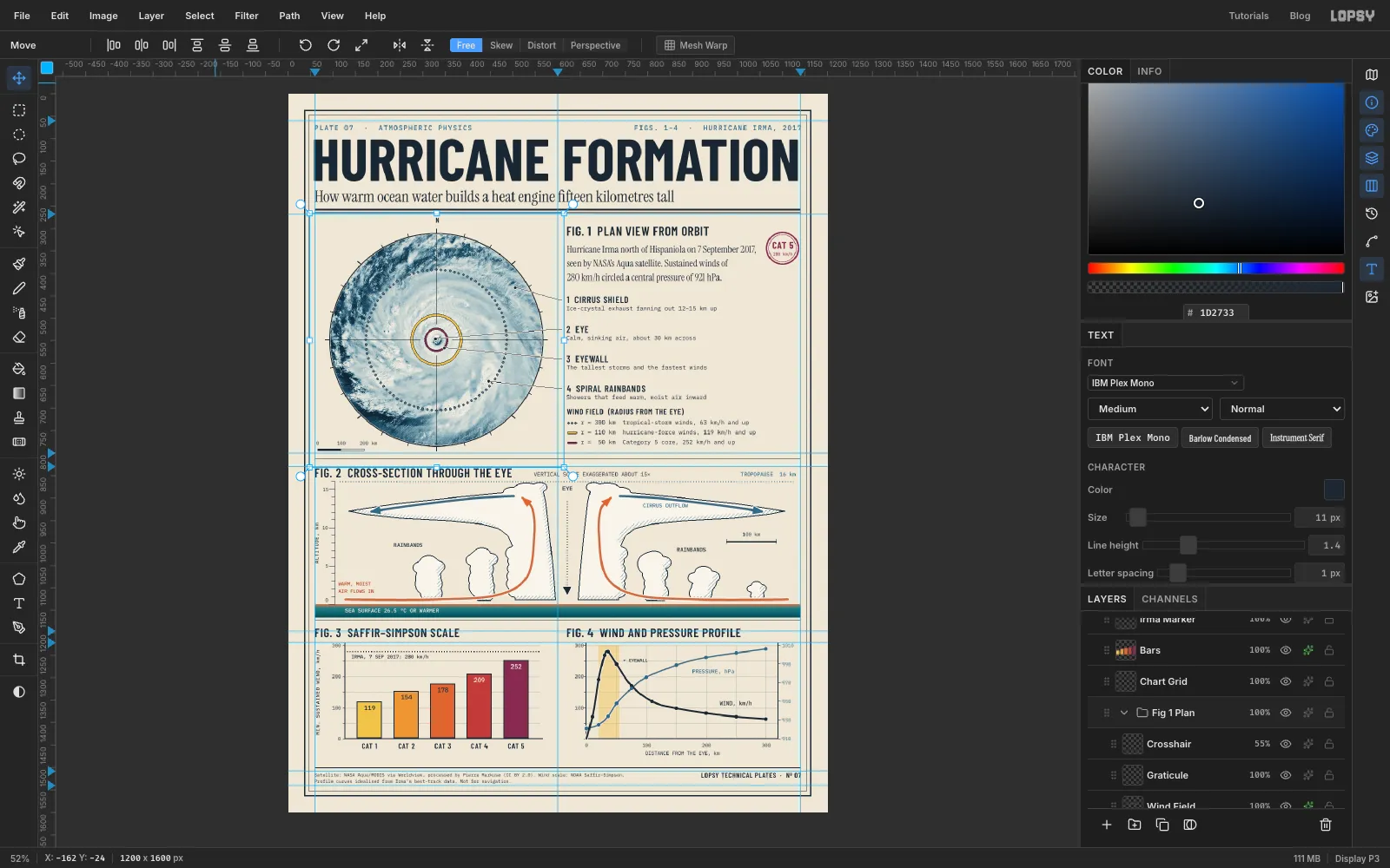
Group each figure
A plate with seventy layers needs some order.
- Click Sea, then Cmd-click every other Fig. 2 layer: the cloud, shade, axis, tropopause, airflow and every Fig. 2 label.
- Choose Layer → Group Layers and name the group
Fig 2 Section. - Do the same with Plan View, Wind Field, Graticule and Crosshair, and name that group
Fig 1 Plan. A group can hold another group, so the duotone keeps working.
Grouping changes nothing on screen: each group goes where its top layer was, and the stacking order stays the same.
-
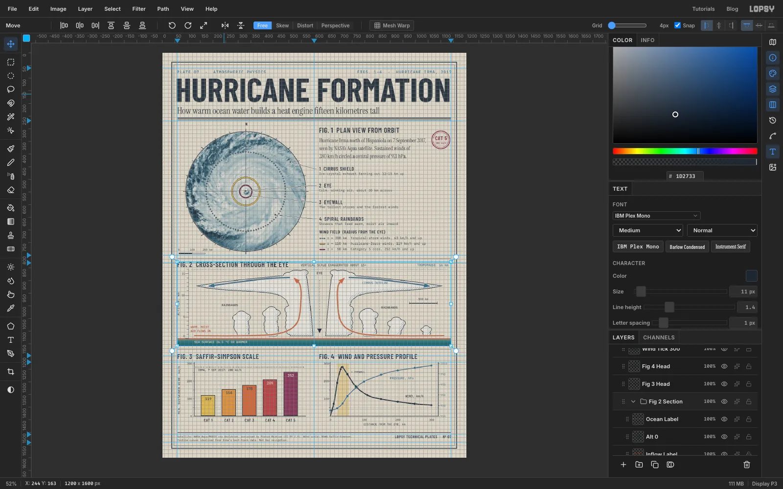
Nudge Fig. 2 into place on the grid
Fig. 2 was built 8 px low. Now centre it between its rules:
- Choose View → Show Grid and drag the Grid slider in the options bar all the way left, to
4px. Check that Snap is ticked. - Select the Fig 2 Section group and pick the Move tool.
- Press Up twice. With grid snap on, each arrow press moves exactly one grid cell, so the whole figure goes up 8 px together. If you go too far, Cmd+Z steps back one press at a time.
- Hide the grid again.
- Choose View → Show Grid and drag the Grid slider in the options bar all the way left, to
-
Add paper grain
One last layer makes the whole plate feel printed.
- Click Title, the headline's text layer, then Add Layer, and name the new layer
Paper Grain. Fill it with mid-grey . - Choose Filter → Add Noise… with Amount
80, Mono and Gaussian. - Set its blend mode to Overlay and its opacity to
60%. Mid-grey disappears in Overlay mode, so only the speckle is left.
The grain sits over the artwork and the headline, while the small labels above it stay crisp.
Choose File → Save Project to keep everything editable, then File → Quick Export PNG for the finished plate.
- Click Title, the headline's text layer, then Add Layer, and name the new layer